Naive Bayes
$\huge Naive\ Bayes$
Naive Bayes is a simple and powerful classification algorithm. It belongs to the family of probabilistic algorithms that take advantage of Probability Theory and Bayes Theorem to predict the class. We calculate the probability of each tag, given the set of input features.

Bird's Eye View of this Blog
- Read and Analyse the Data
- Understanding Law of Total Probability and Bayes Rule using our Dataset as Example
- Applying Naive Bayes on Dataset
Naive Bayes Classifier is based on naïve independence assumptions and Conditional Probabilities. Want to go-over these concepts quickly ? Don't Worry!! We've got you covered. We recommend you reading our blog on Conditional Probabilites. :)
import numpy as np
import pandas as pd
from sklearn.datasets import load_iris
from sklearn.model_selection import train_test_split
import seaborn as sns
import matplotlib.pyplot as plt
from sklearn.preprocessing import LabelEncoder

from IPython.display import HTML
display(HTML('<style>.prompt{width: 0px; min-width: 0px; visibility: collapse}</style>'))
# display(HTML("<style>.container { width:100% !important; }</style>"))
1. Read and Analyse Data
We will use the Iris Flower Classification Dataset.The aim is to classify iris flowers among three species (setosa, versicolor or virginica) from measurements of length and width of sepals and petals. The goal here is to model the probabilities of class membership, conditioned on the flower features.
filepath="Iris.csv"
data_dict=pd.read_csv(filepath)
display(data_dict.head())
display(data_dict['Species'].value_counts())
categories = list(data_dict['Species'].unique())
sns.set(font_scale = 1.2)
plt.figure(figsize=(8,2.5))
ax= sns.barplot(categories, data_dict['Species'].value_counts())
Encoding the labels of Dataset
le=LabelEncoder()
data_dict['Label']=le.fit_transform(data_dict['Species'])
le_name_mapping = dict(zip(le.classes_, le.transform(le.classes_)))
print(le_name_mapping)
display(data_dict.head())
Let us consider the following hypothesis
- H1- The sample belongs to class Iris-setosa
- H2- The sample belongs to class Iris-versicolor
- H3- The sample belongs to class Iris-virgibica
Here the it is assumed that the Hypothesis satisfies following conditions :
- $H1 \cap H2 \cap H3$= NULL
The Hypothesis H1, H2 and H3 are mutually independent. That is a flower strictly belongs to one class. It cannot satisfy two hypothesis at a time.- $H1 \cup H2 \cup H3$= Sample Space
All the data points in our dataset must satisfy any one of the hypothesis.
Calculate Probabilities
Now, we proceed to calculate the probabilities of our Hypothesis based on our Dataset
- P(H1)- Proability of Iris-setosa
- P(H2)- Probability of Iris-versicolor
- P(H3)- Probability of Iris-virginica
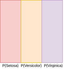
The probabilities can be visualised as follows:
The Hypothesis generates non-overlapping partitions in probability space

Conditional Probabilities
Now, let us assume that our hypothesis is based on the condition C,
- C - The height of the plant is small
From the data we can figure out the following probabilities.
- P(C|H1)- Of the Setosa species, the probability of the plants with small height.
- P(C|H2)- Of the Vesicolor species, the probability of the plants with small height.
- p(C|H3)- Of the Virginica species, the probability of the plants with small height.
Suppose these probabilities are as follows:
- P(C|H1)= 0.1
- P(C|H2)= 0.8
- P(C|H3)=0.7
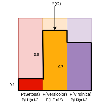
The probabilities can be visualised as follows:

Probability of C can be calculated as : Addition of Areas of 3 Rectangles in Dark Red,Dark Yellow and Dark Purple
\begin{align}
P(C)=(0.3333*0.1)+(0.3333*0.8)+(0.3333*0.7)
\end{align}
\begin{align}
P(C)=P(H1\ \cap\ C)\ \cup\ P(H2\ \cap\ C)\ \cup\ P(H3\ \cap\ C)
\end{align}
Since the sets are disjoint, we can rewrite this as follows:
\begin{align}
P(C)=P(H1\ \cap\ C)\ +\ P(H2\ \cap\ C)\ +\ P(H3\ \cap\ C)
\end{align}
Now, using the definition of conditional probability we can write the intersection as product of two sets as follows :
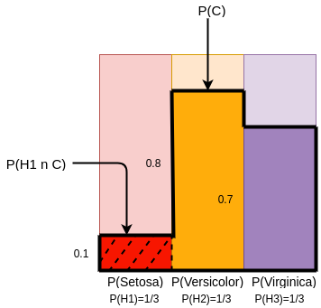
{Geometrical Justification : Area Of Rectangle $P(H1\ \cap\ C)\ =\ Length((P(H1))BreadthP(C|H1))$*}
\begin{align}
P(C)=(P(H1)*P(C|H1))\ +\ (P(H2)*P(C|H2))\ +\ (P(H3)*P(C|H3))
\end{align}
Thus, we have recovered the total probability of C. We did this using Conditional Probabilities of C with three events(Hypothesis) H1,H2,H3.
Now, we ask the inverse question,
Assuming that we know that the plant is small, what are the respective probabilities for plant being Setosa, Versicolor or Virginica?????
2.2 Bayes Rule
In Bayes Rule, if we pick a random sample of iris flower and the condition C (The height of plant is small) is True, then we determine the probabilities of the following :
- P(H1|C) - The small plant sample is setosa
- P(H2|C) - The small plant sample is versicolor
- P(H3|C) - The small plant sample is virginica
To find P(H1|C), we have to find the proportion of intersection of H1 with C to the total area of C

We know that,
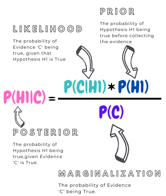
This Gives the Bayes Rule :

3. Applying Naive Bayes on Our Dataset
Step 3.1 Train Test Split
data_train,data_test=train_test_split(data_dict.iloc[:, 1:])
Step 3.2 Calculate Probabilities
def calculate_probability(E,S):
    return float(E/S)
n_total=data_train['Label'].count()

n_setosa=data_train['Label'][data_train['Label']==0].count()
p_setosa=calculate_probability(n_setosa,n_total)
print("The probaility of Hypothesis H1- Sample is Setosa :", p_setosa)

n_versicolor=data_train['Label'][data_train['Label']==1].count()
p_versicolor=calculate_probability(n_versicolor,n_total)
print("The probaility of Hypothesis H2- Sample is Versicolor :", p_versicolor)

n_virginica=data_train['Label'][data_train['Label']==2].count()
p_virginica=calculate_probability(n_virginica,n_total)
print("The probaility of Hypothesis H3- Sample is Virginica :", p_virginica)
Step 3.2 Calculate Likelihood P(C|H1), P(C|H2), P(C|H3)
As we can see here, the features of the data- SepalLengthCm, SepalWidthCm, PetalLengthCm, PetalWidthCm are continuous random variables. A continuous random variable can take infinite number of values within the continuous range of real numbers.
To understand the distribution of random variables, let us visualise using histogram.
features=data_train.columns[:-1]
count=0
fig, axes = plt.subplots(2, 2,figsize=(10,10))
fig.subplots_adjust(hspace=0.3, wspace=0.3)
for i in range(2):
    for j in range(2):
        sns.distplot(data_train[features[count]], hist=True, kde=True,bins=int(180/5), color = 'darkblue', hist_kws={'edgecolor':'black'},kde_kws={'linewidth': 4},ax=axes[i, j])
        count +=1
plt.show()
It is evident that :
- SepalLength, SepalWidth have a Normal Distribution (Unimodal)
- PetalLength, PetalWidth have a BiModal Distribution
We will leverage PDF to model these Random Variables.Probability Distribution Function (PDF)- PDF is a function f(x) of a random variable, x, and its magnitude is an indication of the relative likelihood of measuring a particular value.
Note : For Simplicity, we will use the PDF of Normal Distribution for all the features.
We have to Calculate P(C|H1), we group mean and variances according to the hypothesis.
Calculate Mean
data_means = data_train.groupby('Label').mean()
# View the values
display(data_means)
Calculate Variance
data_variance = data_train.groupby('Label').var()
# View the values
display(data_variance)
Define a Function for Calculating Likelihood Using PDF
# Create a function that calculates p(x | y):
def p_x_given_y(x, mean_y, variance_y):

    # Input the arguments into a probability density function
    p = 1/(np.sqrt(2*np.pi*variance_y)) * np.exp((-(x-mean_y)**2)/(2*variance_y))

    # return p
    return p
Step 3.3 Calculate Posterior Probabilities
def calculate_posterior(features_c,feature_names,prior_prob,num_hypothesis):
    hypothesis_probabilities=np.zeros(num_hypothesis,)
    for i in range(num_hypothesis):

        ##calculate the likelihood by multiplying for all features
        likelihood=1
        for j in range (len(feature_names)):
            x=features_c[j]
            data_mean_x=data_means[feature_names[j]][data_means.index == i].values[0]
            data_var_x= data_variance[feature_names[j]][data_variance.index == i].values[0]
            likelihood= likelihood* p_x_given_y(x,data_mean_x,data_var_x)

        hypothesis_probabilities[i]=prior_prob[i] * likelihood

    return hypothesis_probabilities.argmax()
Step 3.4 Predict on Test Data
def calculate_test_prediction(data_test,prior_prob,num_hypothesis,feature_names):
    data_test_pred = []
    count=0
    for i in range(len(data_test)):
        features_c=data_test.iloc[i,:-2]
        y_pred=calculate_posterior(features_c,feature_names,prior_prob,num_hypothesis)

        data_test_pred.append(y_pred)
        if(y_pred==data_test['Label'].iloc[i]):
            count+=1

    accuracy=float(count/len(data_test))*100

    return data_test_pred,accuracy
data_test_pred,acc=calculate_test_prediction(data_test,[p_setosa,p_versicolor,p_virginica],3,data_means.columns)
acc